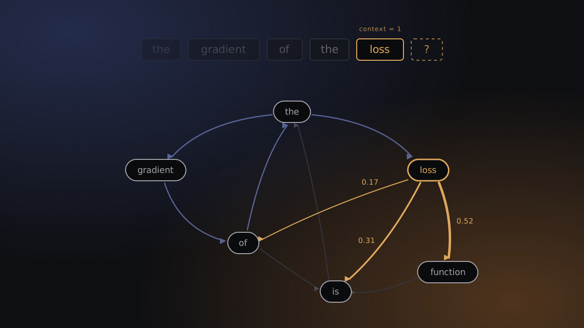
This LLM has a Context window of 1
Exploring the basics of LLMs by training a N-Gram model on my lecture notes
100% Human-written
Introduction
An n-gram model analyzes training data to determine how frequently specific word sequences occur. For example, given the phrase “my house is,” the model examines all words that follow “my” in the dataset. If “house” is the most common continuation, the model predicts “house.”
In this Post, I will cover the mathematical basics of modern LMs and train my own N-Gram Model based on my lecture notes. I’ll take a mathematical dive into different token selection functions and prove why the maximum likelihood assumption leads to periodic repetition.
Mathematical Basics
This section is largely based on the book Speech and Language Processing by Jurafsky & Martin (2026, I.3)
Most language models use context consisting of tokens to predict the nth token and describe the probability for every next token with . N-Gram models limit this context by assuming . In the extreme case of a bigram model () this assumption simplifies to , we call this the markov assumption. The probability of outputting a sentence with token-length based on context token is . I define as the set of all sentences with length N. And We define as the number of occurrences of with the sentence preceeding. The next token selection is decided by .
In our case, we define , simplifying to with bigrams.
Greedy decoding always ends in a loop
Let’s take the maximum likelihood assumption of picking with .
Before we improve , let’s prove why choosing greedily will fail.
Proof
Adapted from Knuth (1997)
We define a greedy as:
Given vocabulary with : Generation from a seed is then nothing but iterating:
Theorem. For every the greedy sequence is eventually periodic: there are where such that , and the sequence repeats with an arbitrary period :
Proof. Look at the first tokens . They are elements drawn from a set of only tokens, so by the pigeonhole principle two of them must coincide: for some . Because is a function:
So the sequence is periodic with period from index on.
What do we learn from that?
- Repetition is structural, not a bug of the dataset. Any finitely large dataset doesn’t fix the underlying problem.
- The model can produce at most distinct texts
- Termination is luck. We can’t guarantee the loop contains a EOS.
Markov
To prevent this, we sample from . Thus, is no longer a function, but a stochastic kernel of a markov chain. This leads to the key insight that a bigram model with this is equivalent to a markov chain, where nodes are tokens and edge weights are .
We can also model higher-order N-Grams as markov chains, where the number of nodes increases exponentially with .
The better selection Funct
This section is based on Jurafsky & Martin (2026) too
The maximum likelihood assumption fails in the real world. No matter how big the training set, some sentences will never be able to be generated. That leaves the model locked on a subset of real language.
One option is Laplace Smoothing:
This leads to this Prediction function in bigram models:
Laplace charges a proportional tax on evidence
What count would have produced this probability without smoothing? Solving for gives the effective count
That factor is brutal at the vocabulary sizes we are dealing with. My vault has types, and a decently frequent context like Gradient might have . Then , and the bigram Gradient Descent, observed 50 times, ends up with an effective count of roughly . We spent a whole corpus collecting that evidence and then threw away of it to fund continuations that never happened.
Lets add more!
Add- smoothing, , only changes the tax rate. The structural problem survives: the amount of mass taken from observed events scales with and with nothing about the context except its total count. A single tuned on held-out data is always a compromise between contexts we know a lot about and contexts we saw three times.
Discount, don’t rescale
Both scale multiplicatively. But held-out counts show the MLE error is additive: bigrams seen times recur about times (2026). So subtract a fixed instead. Normalization then forces the freed mass to be
so diverse contexts leak more. It is only consulted in unseen contexts, so count how many distinct contexts appears in, not how often. Descent is frequent, yet almost always follows Gradient.
Knesner-Ney
We arrive at Knesner-Ney. The right term spends exactly the deficit the left one creates. is normalized, so is freely chosen.
Perplexity
For LM evaluation, we use Perplexity. It is the exponentiated average negative log-likelihood the model assigns to held-out text:
Read it as an effective branching factor: how many words is the model effectively choosing between at each step? A uniform model over my vocabulary has a perplexity of exactly 15,622, because it is choosing uniformly between 15,622 options. Lower is better (Jurafsky & Martin, 2026).
Building an N-Gram Model
I was able to extract 585 .md files, skipping the following:
forbidden = [
    r"*/.claude/*",
    r"*/.obsidian/*",
    r"*.excalidraw.md",
    r"*/node_modules/*",
]
Preprocessing: Markdown is not prose, since markup is far more repetitive than text, so a model trained on the raw vault would spend most of its probability mass learning that [ follows ]. Twenty-one ordered regex substitutions normalise this, anything carrying display text is reduced to it (aliased wikilinks, markdown links, callout headers), anything else is deleted rather than replaced (frontmatter, code, math, embeds, URLs, HTML, hashtags, rules). Pure markers (headings, bullets, blockquotes, checkboxes, emphasis) are stripped. Because a lecture note is a stack of grammatically unrelated bullet fragments, each line becomes its own training sequence. All exact duplicate notes are dropped by content hash, since the same content being in training and validation set would defeat the point.
| markdown files | 588 |
|---|---|
| after deduplication | 533 |
| non-empty documents | 388 |
| training tokens | 277,208 |
| held-out tokens | 11,023 |
| types → vocabulary | 23,988 → 15,622 (96.98% coverage) |
277k tokens is very small. For scale, GPT-3 was trained on roughly 300 billion.
How much context is worth paying for?
So I trained one model per order, from (uniform) up to , and measured each on the same held-out documents:
| N | 0 | 1 | 2 | 3 | 4 | 5 | 6 | 8 | 10 | 12 | 15 | 19 |
|---|---|---|---|---|---|---|---|---|---|---|---|---|
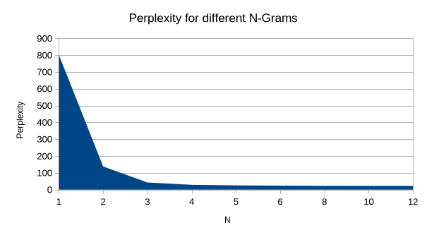
| Perplexity | 15622 | 801 | 137.8 | 42.6 | 28.8 | 25.5 | 24.0 | 22.8 | 22.5 | 22.5 | 23.0 | 23.9 |
Improvement seems to be lorarithmic. The “context window of 1” divides perplexity by almost six, and the trigram cuts it by another two thirds. After perplexity doesn’t seem to improve.
Later it surprisingly goes back up. Past , more context makes the model measurably worse. This seemingly is because it has fewer training data for longer lines. At , 15% of held-out tokens arrive with a context the model has never seen; by it is 35%.
What it actually writes
Perplexity doesn’t paint the whole Picture. So a test run: same seed, same prompt, one model per order:
--- N = 1 ---
the main
 of
: ,
:
.
 . 1
 the 3 the , b
die

--- N = 2 ---
the main process
:
for all
x lecture 03 .
removed and the
in order to a basis of b ,
fixed a 4 , then there is true .

--- N = 3 ---
the main process before processes are launched when using a kernel , the
removed property from the other files : , email 42 , concat name , :
the trainer no longer randomly selects a seed no longer returns a triplet 18390
: there is a subset of examples for pytorch 2.4 .
if is even .

--- N = 5 ---
the main academic risks are : unclosed gaps in securityprivacy weeks 14 15 , the rsa calculation error , and the missing .
you can decompress drawing data with the command palette : decompress current excalidraw file .

--- N = 10 ---
the main academic risks are : unclosed gaps in securityprivacy weeks 14 15 , the rsa calculation error , and the missing buffer-overflow payload practice .
a graph is planar if it can be drawn on a paper such that no edges cross each other
Every line break is the model emitting </s> and starting a fresh sequence, so the number of lines is itself a signal: the higher the order, the longer it keeps going before it decides EOS.
is function words and punctuation — the model has no context, so it produces the most common tokens in the language, which are the ones carrying no meaning. is the interesting one: locally grammatical, globally nonsense. “the main process before processes are launched when using a kernel” actually quite good, you’d have to secondguess to figure out it is nonsense.
And then and stop writing and start quoting. “A graph is planar if it can be drawn on a paper such that no edges cross each other” is a line from my notes on discrete modelling, reproduced word for word.
The minimum is a lie
That is just an impression though, so let’s measure it. For each order I sampled a few hundred lines, cut them into 8-grams, and checked how many of those 8-grams appear word for word in the training split and, separately, how many of the generated lines are entire lines of the vault reproduced exactly:
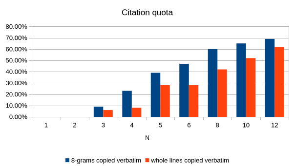
The rows move together. Every point of perplexity I bought past was paid for in originality: at the perplexity minimum, two out of three 8-word spans the model produces are copied straight out of my notes, and half of the lines it writes are completely out of my notes.
At , 62% of the contexts the model knows occur exactly once in the entire corpus. The model isn’t choosing. It is looking up the rest of the line.
Which brings us back to its own proof. Greedy decoding fails because it is a function on a finite set, so it must eventually cycle. Sampling fixes that, but at high it stops repeating itself and starts repeating me. Both are a model with nothing of its own to say, and only the first one is visible in the loss.
If you want the most original model, I suggest or : still recombining, just before the counts get sparse enough to overfit. → The best-scoring model and the best model are not the same.
One model, two languages
My notes are bilingual, and both go into one model with one vocabulary. So it code-switches mid-line, as I do in my notes:
fixed an issue to avoid validation loop : : set aller möglichen hypothesen nach der hypothesis
der lokale daemon muss als eigenständige for any
Improvement opportunities
- Estimate the discount instead of guessing it. is hard-coded to 0.75 throughout. Let’s change that and use a separate delta for N=1,2,3+: (2026).
- Top-k sampling. We could store the k most next and , normalized such that in a key-value store and run the Markov kernel only on those fixed number of tokens. This would mean Inference goes from per token to , independent of vocabulary and order. Note that this isn’t a lossless operation (Fan et al., 2018).
Limitation
There is a ceiling, and it is not an engineering problem. An n-gram model stores a table indexed by context, so its parameter count grows as . With my modest 15,622-token vocabulary, a 10-gram table has cells. I observed 277,208 of them. Every additional token of context multiplies the space by 15,622 and adds zero new evidence.
That is the wall the whole field hit, and the reason the next idea had to be structurally different rather than merely bigger. This ceiling was already visible in the smoothing literature by 2001 (Goodman, 2001), and still standing in 2007 when Google trained 5-grams on two trillion tokens of web text and watched the gains go logarithmic.
Conclusion
So: what does a context window of 1 get you? A perplexity of 137.8, sentences that are grammatical for about four words at a time, and a model small enough an Arduino would be able to run it easily.
It doesn’t get you anywhere near the level of competence modern LLMs have and finds no relation between similar tokens. You can’t embed tokens or find any semantically valuable information in the models.
References
- Fan, A., Lewis, M., & Dauphin, Y. (2018). Hierarchical Neural Story Generation. https://arxiv.org/abs/1805.04833
- Goodman, J. T. (2001). A bit of progress in language modeling. Computer Speech & Language, 15(4), 403–434. https://doi.org/10.1006/csla.2001.0174
- Jurafsky, D., & Martin, J. H. (2026). Speech and Language Processing: An Introduction to Natural Language Processing, Computational Linguistics, and Speech Recognition, with Language Models (3rd ed., I.3). https://web.stanford.edu/~jurafsky/slp3/
- Knuth, D. E. (1997). The Art of Computer Programming, Volume 2: Seminumerical Algorithms (3rd ed.). Addison-Wesley.
- Ney, H., Essen, U., & Kneser, R. (1994). On structuring probabilistic dependences in stochastic language modelling. Computer Speech & Language, 8(1), 1–38. https://doi.org/https://doi.org/10.1006/csla.1994.1001